반응형
import numpy as np
import pandas as pd
import matplotlib.pyplot as plt
import seaborn as sns
%matplotlib inline  #노트북안에서 바로 그래프를 출력하여 보여줌

import warnings
warnings.filterwarnings('ignore')

#데이터 불러오기
datapath = 'https://github.com/mchoimis/tsdl/raw/main/income/'
df = pd.io.parsers.read_csv(datapath + 'income.csv')
df.head()

# 데이터 형태 확인
print(df.shape)
print(df.columns)
df.info()

# 결측치(NA, 없는 값)를 NaN으로 바꾸기
df[df=='?'] = np.nan
df.head()

# 최빈값으로 결측치 채우기
for col in ['workclass', 'occupation', 'native.country']:
    df[col].fillna(df[col].mode()[0], inplace=True)
    #선택한 열(column)에서 가장 자주 나타나는 최빈값(mode) 중 첫 번째[0] (참고 median 중간값)

df.isnull().sum()

X =  df.drop(['income', 'education', 'fnlwgt'], axis = 1)
y =  df['income']
원 데이터를 training set과 test set으로 나누기
from sklearn.model_selection import train_test_split

X_train, X_test, y_train, y_test =  train_test_split(X, y, test_size = 0.3, random_state = 0)
범주변수 처리는 2가지
- 클래스를 숫자로 변환
#LabelEncoder
#예시1
from sklearn import preprocessing

le = preprocessing.LabelEncoder()
le.fit(["red", "green", "blue"]) # 라벨 정보 학습
print(le.transform(["red", "red", "blue", "green"])) # 데이터 변환

#예시2
from sklearn import preprocessing

categorical = ['workclass', 'marital.status', 'occupation', 'relationship', 'race', 'sex', 'native.country']
for feature in categorical:
        le =  preprocessing.LabelEncoder()
        X_train[feature] =  le.fit_transform(X_train[feature])
        X_test[feature] =   le.transform(X_test[feature])
        # train으로 라벨인코더를 한 후 test에서 동일한 매핑을 사용하여 범주형 값을 나누기 위함.
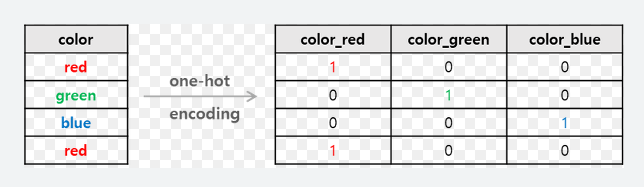
- 원-핫 인코딩(더미코딩)
(참고) scikit-learn에서 제공하는 피처 스케일러(scaler)
- `StandardScaler`: 기본 스케일, 각 피처의 평균을 0, 표준편차를 1로 변환
- `RobustScaler`: 위와 유사하지만 평균 대신 중간값(median)과 일분위, 삼분위값(quartile)을 사용하여 이상치 영향을 최소화
- `MinMaxScaler`: 모든 피처의 최대치와 최소치가 각각 1, 0이 되도록 스케일 조정
- `Normalizer`: 피처(컬럼)이 아니라 row마다 정규화되며, 유클리드 거리가 1이 되도록 데이터를 조정하여 빠르게 학습할 수 있게 함

알고리즘 구현
# Feature scaling 전 원본 데이터
from sklearn.linear_model import LogisticRegression
from sklearn.metrics import accuracy_score
#accuracy_score는 분류 문제에서 모델의 예측 결과와 실제 레이블을 비교하여 정확도를 계산하는 함수

logreg =  LogisticRegression()
#LogisticRegression() 함수는 fit()사용하여 모델 학습, predict()사용하여 데이터 결과 예측
logreg.fit(X_train, y_train)
y_pred = logreg.predict(X_test)

# logreg_score =  accuracy_score(y_test, y_pred)
print('Logistic Regression accuracy score: {0:0.4f}'. format(accuracy_score(y_test, y_pred)))
스케일이 조정된 알고리즘 구현
# Feature scaling 후 변환 데이터
from sklearn.linear_model import LogisticRegression
from sklearn.metrics import accuracy_score

logreg = LogisticRegression()
logreg.fit(X_train_scaled, y_train) #스케일 조정'scaled'
스케일 조정된 데이터를 이용한 Logistic Regression 모델 분류결과 확인하기
from sklearn.metrics import classification_report

cm_logreg_scaled_data =  classification_report(y_test, y_pred_scaled_data)
print(cm_logreg_scaled_data)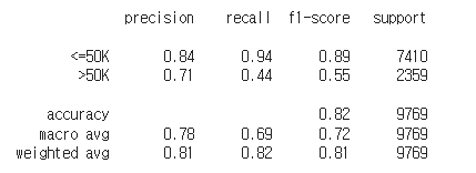
*f1-score는 다음에
Random Forest 모델 구현하고 정확도 확인하기
from sklearn.ensemble import RandomForestClassifier  #ensemble모델 中 RandomforestClassifier
from sklearn.metrics import accuracy_score

rfc = RandomForestClassifier()
rfc.fit(X_train, y_train)

# 분류 모델 하이퍼 파라미터 예시
criterion='gini' # The function to measure the quality of a split. Supported criteria are “gini” for the Gini impurity and “entropy” for the information gain (정보 이득)
n_estimators=100 # The number of trees in the forest.

y_pred = rfc.predict(X_test)
rfc_score =  accuracy_score(y_test, y_pred)
print('Random Forest Model accuracy score : {0:0.4f}'. format(rfc_score ))
Random Forest Model accuracy score : 0.8475
Random Forest 모델의 Confusion Matrix 확인하기
from sklearn.metrics import confusion_matrix

cm =  confusion_matrix(y_test, y_pred)
print('Confusion Matrix for Binary Labels \n')
# print('Confusion Matrix for Binary Labels\n')
# print('Actual class')
# print('Predicted', '[[True Positive', 'False Positive]')
# print('         ', '[False Negative', 'True Negative]]')
print(cm)

# Confusion Matrix에서 Recall과 Precision 계산하기

print('\nRecall for Class [<=50K] = ', cm[0,0], '/' , cm[0,0] + cm[0,1])
print('\nPrecision for Class [<=50K] = ', cm[0,0], '/' , cm[0,0] + cm[1,0])
print('\nRecall for Class [>50K] = ', cm[1,1], '/' , cm[1,0] + cm[1,1])
print('\nPrecision for Class [>50K] = ', cm[1,1], '/' , cm[0,1] + cm[1,1])


#결과확인
from sklearn.metrics import classification_report

cm_rfc =  classification_report(y_test, y_pred)
print(cm_rfc)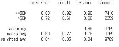
Gradient Boosting 모델 구현하고 정확도 확인하기
from sklearn.ensemble import GradientBoostingClassifier

gbc =  GradientBoostingClassifier(random_state=0)
gbc.fit(X_train, y_train)

y_pred =  gbc.predict(X_test)
gbc_score =  accuracy_score(y_test, y_pred)
print('Gradient Boosting accuracy score : {0:0.4f}'.format(gbc_score))

from sklearn.metrics import classification_report

cm_gbc =  classification_report(y_test, y_pred)
print(cm_gbc)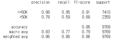
Light GBM 구현하고 정확도 확인하기
from lightgbm import LGBMClassifier
from sklearn.metrics import accuracy_score

lgbm =  LGBMClassifier(random_state=0)
lgbm.fit(X_train, y_train)
y_pred =  lgbm.predict(X_test)

lgbm_score =  accuracy_score(y_test, y_pred)
print('LGBM Model accuracy score : {0:0.4f}'.format(lgbm_score))

from sklearn.metrics import classification_report

cm_lgbm =  classification_report(y_test, y_pred)
print(cm_lgbm)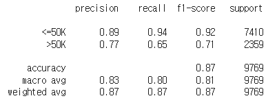
요약
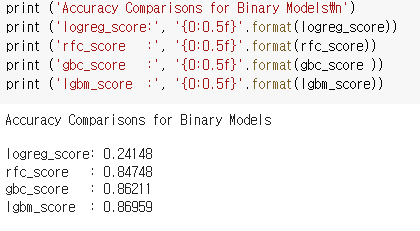
logistic Regression은 일부 오류 있는 듯
출처: 패스트캠퍼스
반응형
'코딩 > Python' 카테고리의 다른 글
| [파이썬] 혼자 공부하는 데이터 분석(03-2 잘못된 데이터 수정하기) (0) | 2023.04.25 |
|---|---|
| 웹스크래핑(교보문고 ISBN으로 쪽수 가져오기) (0) | 2023.04.23 |
| 파이썬, openpyxl(6) 수식작성, 병합, 이미지삽입 (0) | 2023.03.31 |
| [Python] 백준 6603 로또 (0) | 2022.12.29 |
| [Python] 백준 10819 차이를 최대로 (0) | 2022.12.29 |